An Intuitive Description of Runge-Kutta Integration

(Based on a StackOverflow answer from November 2009)

Introduction

This may be a bit oversimplified so far as actual math, but is meant as an intuitive guide to how Runge Kutta integration works. RK integration is a numerical method for solving arbitrary first-order differential equations widely used by scientists, engineers, video game programmers, and everyone else who uses applied math beyond the simple.
Suppose we want to predict or simulate some physical system measured by some quantity y varying with time, y(t), for which we have an equation giving its rate of change

y'(t) = f(t,y)

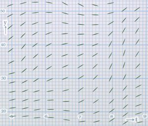
For any time t and any value of y, the (simulated) forces or activities of the system determine a unique slope.

Slopes are given at every point in (t,y) space.

The function f(t,y) may be a simple algebraic function of t and y, or it may be a messier expression with exponentials and square roots and many terms. It may involve interpolating values given in a table. It may involve real-time data pouring in from gyrscopes, strain guages, photodiodes or other sensors.

Integration

With this kind of first-order differential equation, we are usually given an inital value y1 at some time t1. We want to know y at some later time t2.
From the differential equation, we can find the rate of change of y at t1. There is nothing else we can know for sure; everything else from here onward is guessing. We want to do a very good job of guessing.

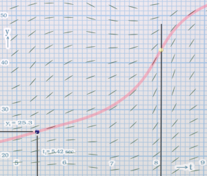
Setup of the basic integration problem. Try to find the value of the pink curve at t2, when you don’t already have the pink curve.

We cheat a bit here, and show the exact solution in pink. This will help us to judge how values computed numerically deviate from the ideal. In real life, we almost never have an exact solution to look at.

Euler integration is the simplest way to guess the future: linearly extrapolate from t1 to t2, using the precisely known slope and value of y at t1. This usually gives a bad answer. If t2 is far from t1, the linear extrapolation will fail to match any curvature in the ideal solution. If the step is too large, we might miss an intersting change in slope, an inflection point, or something. If we try to follow the ever-changing slopes more closely by taking many small steps from t1 to t2, we’ll have the problem of subtraction of similar values, resulting in roundoff errors, and it’ll take far more computational work to get to t2.

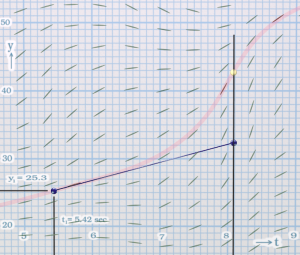
Euler integration: One big linear extrapolation step determined only by information at the initial point. Euler sux!

If the differential equation happens to be very simple, like dy/dt = constant, cool, we actually have an exact answer. Real life is always more interesting than that and often nonlinear.
So we refine our guess. One way is to go ahead and do this linear extrapolation anyway, then hoping it’s not too far off from truth, use the differential equation to compute an estimate of the rate of change at t2. This, averaged with the (accurate) rate of change at t1, better represents the typical slope between t1 and t2 (shown in red below). We use this to make a fresh linear extrapolation from to t1 to t2. It’s not obvious if we should take the simple average, or give more weight to the more accurate slope at t1, without doing the math to estimate errors. Just note that there is a choice here. In any case, it’s a better answer than Euler gives.

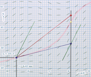
How to do better than Euler: Take one normal Euler step (blue). Find the slope at t2 (green) and compare wih the initial slope (blue). Find their average for a “better” full step to t2 (red).

Making Half the Effort

Perhaps better, make our initial linear extrapolation to a point in time midway between t1 and t2, and use the differential equation to compute the rate of change there (blue). This gives roughly as good an answer as the average just described. Then use this mid-way slope for a better linear extrapolation from t1 to t2, since our purpose is to find the quantity at t2. This is the midpoint algorithm. It’s really no better than Euler.

Finding the y value and slope at the midpoint depends on the slope at the initial point. We’d like to not be starting off in the wrong direction. What if we use this rough mid-point slope to make another linear extrapolation from t1 to the midpoint t? This is the red line in the figure below. It’s the same slope as the blue line, but relocated to the initial point t1,y1. With this, the differential equation gives us a better estimate of the slope at the halfway point. This lets us extrapolate once again from t1 all the way to t2 for a truly better answer. This is the Runge Kutta algorithm, at least a simple form of it.

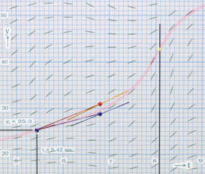
Maybe the slope at halfway across is better than averaging the initial and estimated final slope? Our first midpoint attempt (blue) can be used to obtain a better position at the midpoint (red and gold).

Could we do a third extrapolation to the midpoint? Sure, it’s not illegal, but detailed analysis shows diminishing improvement, such that other sources of error dominate the final result.

After that, we may compute the slope at t2, and somehow use that to better estimate how the the values and slopes of the ideal solution change with t. At this point, wordy hand-waving arguments and colorful sketches aren’t going to help. We need to do the algebra for fitting low-order polynomials to the values and slopes found by methods like we’ve described. Linear extrapolations and averages can only go so far. For true gains in quality we must consider 3rd and 4th order polynomials and tweak the details to obtain minimal errors.

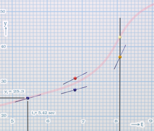
The fourth-order RK computes slopes at four locations. Each location was determined from previous locations and their slopes.

 

Runge-Kutta Choices

The most popular form of fourth-order Runge Kutta uses the differential equation to compute the slope four times:

1. at the intial point t1,
2. twice at two in-between points,
3. once at the final point t2.

The location of the in-between points are a matter of choice. We’ve illustrated having both at the midway point between t1 and t2. It is possible to choose points elsewhere, for example at one third of the way along and another at 2/3 of the way. The weights for averaging the four slopes will be different. In practice this doesn’t change things much, but may work slighty better for certain applied problems. Comparing different R-K algorithms applied to the same differential equation and initial data has a place in testing since, within errors that can be estimated, answers ought to agree.

Higher Orders, Lower Orders

Euler’s method is actually a first-order Runge Kutta method. R-K covers a range of methods to choose from. You don’t want first-order, as every beginner at numerical integration discovers from experimenting with Euler. Higher order methods are better, up to fourth order. Beyond that, the extra effort rarely pays off in performance.

Remember that beside the integration method, there is the choice of step size. Higher order RK methods allow you to take longer steps, therefore fewer steps. While there’s more computational work at each step, it’s less work overall to get from t1 to t2.

Original Inspiration

The essence of the  original question, which won a  Notable Question badge, is:

Can anybody explain in simple terms how RK4 works? Specifically, why are we averaging the derivatives at 0.0f, 0.5f, 0.5f, and 1.0f? How is averaging derivatives up to the 4th order different from doing a simple euler integration with a smaller timestep?