A Review of Build Systems, 2015

To study waves, one must calculate. To calculate requires creating software. If it’s not simple, a build system and souce control system help keep things straight.

Every few years I look over the landscape of build systems to see what’s new, what’s different, and if I might like to choose a different favorite for my own general use and to recommend for projects at work.

Peeking ahead, The Conclusion: CMake is the winner in most cases, with QMake a close second if there’s only one target.

Sometime around ten years ago I chose Peter Miller’s Cook for personal projects because it seemed elegant, useful, and solved some problems of using plain Makefiles.   For a large project containing several executables, several libraries, user documentation and technical documentation, it is common to have a Makefile, or whatever files a build system uses, for each of those components, and a master file to invoke them.  This is done all the time with Makefiles. But there are problems with that – conveying values of variables, having to repeat dependencies, lists of linker options, and so forth, and worst of all, having to re-determine file obsolescence over and over as each Makefile determines the work needed for its target.   Cook solved some of those problems, as did several other newer build systems.   What is desired, ultimately, is to spend little time on build system activities compared to actually compiling and linking.  In particular, a null build (when all target files are up to date) should run “quick” which for most us, should be just a few seconds if not in an apparent instant.

The key paper on this, “Recursive Make Considered Harmful” by Peter Miller, is required reading for all computer scientists, software engineers, and science-math-art types like me who pretend to be such.  It can be found in numerous places on the WWW.

Another important characteristic of a good build system is platform independence.  Make and Cook both fail at this, due to using shell commands for carrying out build steps.   It is impossible to write a command to compile on Linux or BSD, and have it also work on Mac, and also on Windows, and also on all the popular embedded systems.   This is not just a matter of hiding “gcc” or “clang” or “CL” behind a macro $(CC) along with their more common options.    Abstraction to the point of telling the build system to “compile” a .cpp file to get an object file (and we don’t have to say if it’s “.o” or “.obj”) allows platform-independent builds.

Along with this, is the fact that most Windows developers like to use MS Visual Studio.  Most linux/unix developer are happy with a command line, though a variety of IDEs could be in use.  Java and Android developers tend to use Eclipse.  Abstraction of specific commands into named concepts allows the build system to produces artifacts that aren’t command-based, such as IDE project files, and files for less abstract build systems such as Makefiles.

This sort of build system, highly abstract and which produces files for simpler build systems,  could be called a Second-Order Build System.  These seem to be the winning technique throughout industry.  CMake excels at this.

CATEGORIES of BUILD SYSTEMS

* Simple direct build systems

:  Make, Cook, Rake. Often limited to few platforms, specific toolchains.  Easy to learn, use, test. Horrible once you want to scale up or spread to other tools, platforms.

Main benefit is these are easy to learn, having a simple basic working principle.

Easy to set up for tiny projects, as long as you don’t want portability.

Fine for in-house one-off projects.

* Powerful Self-Contained Build Systems

, providing abstraction and portability, which do all the work themselves such as finding platform-dependent libraries, fiddling with paths, invoking compilers.  Scons is an example.

* Second-Order Build System

, also abstract and portable, but don’t do the work themselves.  Instead these systems degate the blue-collar work to simpler build systems, which is nearly always Make. A second-order build system creates Makefiles or IDE project files.  Beware the dangers of Recursive Make. Widely used examples: QMake, CMake.

* Specialized Build Systems

– just for a certain language, maybe only on a specific platform.  Unlike the Simple Direct Build Systems, these don’t even pretend to be portable or abstract.  Fine for academic exploration, specialized embedded systems, cutting edge new hardware.   Use one of these if necessary, but otherwise avoid. Not discussed further in this article.

* No Build System

.  Some languages such as the “scripting” ones, like Python, Perl do not need compiling.  A byte-code compiled file may be created by the interpreter, but is handled entirely by the interpreter. It is hardly a build system. In other cases, no build system is fine for students writing “hello world”, researchers trying out experimental compilers, and offbeat platforms lacking a normal set of tools.

REQUIREMENTS and DESIRED CHARACTERISTICS of a GOOD BUILD SYSTEM

Popularity

* Well established, well-used. We can rely on it for mission-critical work, company jewels.  Must have escaped its crib of origination, gotten into the hands of many users with no connection with the inventors.   Exception: for those who love intellectual adventures, debugging, and have ample spare time for writing and submitting patches, then never mind. This exception is not applicable to me or anyone I know.
* Good documentation, good online support, widespread know-how.  We do not want to be often scrutinizing the build tools’ source to figure out how to use it.
* One way to see if a tool has popularity, support, and community is to run a half-hearted superficial Google search. (Or a duck-duck-go search.)  When not trying hard, success stories, blogs, tutorials and more should come up anyway.   This is evidence that the tool has escaped its crib.

Logic and Efficiency

* Can build just one component of a large system.   If the source control allows it, a developer should be able to pull just one major component with its dependencies, compile it, debug it, and submit changes.  Some build systems insist on running only from the top level.
* Quick null build (all files already up to date)
* Multiple out-of-tree builds (diff CPU, demo/real, debug/release, ..)
* Faster is better than Slower.  (Duh!)
* Not cumbersome for tiny projects.

Targets and Development Environments

* Can build on and target Windows, Linux, with future targets that may include OSX, iOS, Android, various embedded systems.
* When building on Windows, can create files for Visual Studio.
* On Mac, files for XCode.
* There is no IDE of choice on Linux, but perhaps support for Eclipse would be nice – if only as an indication that the tool can support a wide variety of development environments.

Toolset flexibility

* Choice of compiler: gcc vs clang.  Could we use clang for  Windows projects? Sure, anything is possible these days, but how easy will it be to support stunts like that in the build system?
* No hand-writ dependencies  (like xxx.c : xxx.h  common.h seen in Makefiles) (but can be done if necessary)
* Easy to incorporate external library, component, etc w/o much fuss.
* While C, C++ will be our main languages, should not be confined to working with those.

Installation and Ramping Up

* Using the build tool does not require installing forty other things, esp not obscure languages, libraries which in turn drag in tons of stuff
* Easy for an experienced developer, not expert on the build system, to figure out how to use it for a typical medium-sized project.

WORTHY CANDIDATES

With comments, evaluations, links. Highly biased, based on my limited knowledge and search time.

GNU Make

Simple direct build system based on famous old unix ‘make’.
Very unix/linux oriented. Uses shell commands.
Original make on unix created 1970s, grew popular long ago, now universal.
http://www.gnu.org/software/make/  – current
GNU license.

GNU Autotools = Autoconf, Automake

Tools to generate Makefiles, adapting them to specific machines according to 32/64 bit, availability of libraries, optimization levels.
Widely used for GNU and other open source projects.
Messy system that grew over time into rat’s nest of detail.
Difficult to learn.  Very unix/linux oriented, shell commands.
Only build system for which the word ‘arcane’ is used.
http://www.gnu.org/software/automake/   – current
https://autotools.io/index.html  (2013)
GNU license.

CMake

Second-Order Build System, covering all significant platforms, architectures.
From ITK, maker of VTK 3D data visualization software.

Though it creates recursive makefiles on linux, the problems with that are anulled
because cmake stays in charge during dependency checks, writes clever makefiles.

Used by many large projects, open source and proprietary.
I am familiar with CMake for NRAO’s CASA radio astronomy software. It worked well.
CMake is used by ROOT, the major software tool used for high energy physics at CERN.
Used by:  OpenCV, Point Cloud Library,  zlib, Armadillo, OGRE 3d engine

Can build an individual target, but by name at top level,
not by cd’ing down and building there.
Created ~2000, grew within science and 3D graphics community,
then mid-2000s started catching on more widely.
http://www.cmake.org/   – current
http://aosabook.org/en/cmake.html

QMake

Second-Order Build System.
Primarily for Qt-based C++ projects, requiring special preprocessing.
Can be used for non-Qt projects, but this is rarely done.
Easy to learn, get going on small projects.
Simple clean language. Add source file with elegant lines like
HEADERS += foo.h
SOURCES += foo.cpp

Deal with common conditional situations with code like
!exists( main.cpp ) {
error( "No main.cpp file found" )
}
win32 {
SOURCES += win32demoscreen.cpp
}

Easy to deal with platform variations, since Qt already aims to be cross-platform.
But its biggest flaw: makes only one target per *.pro file.  It is possible
to have many .pro files, and have QMake create as many Makefiles, with a master
Makefile to rule over them, but it is not clear to me if this is a good idea. Also,
one may define multiple “configurations” in one .pro, each providing one target, but
you must manually run qmake once for each config.
http://doc.qt.io/qt-5/qmake-overview.html
https://blog.qt.io/blog/2009/10/12/to-make-or-not-to-make-qmake-and-beyond/

Boost.Build

Created for Boost libraries.
Handles all platforms of interest, variety of toolchains. Since the Boost libraries
strive hard for universal portability, it makes sense their build tools would follow.
http://www.boost.org/build/index.html
Boost License

Scons

Python-based direct build system.
Was used by NRAO for CASA, until they switched to CMake.
(Parts are still scons, or have scons and cmake as redundant build systems.)
Good at handling many files spread over complex directory tree, with
the resulting file much smaller than equivalent Makefiles, perhaps 1/4 to 1/10th size.
Weak at IDE support – does not create .proj etc but instead, you must teach
your IDE (VS, XCode or whichever) to run scons as an external command or script.
see https://bitbucket.org/scons/scons/wiki/IDEIntegration
Even so, just isn’t nice with Windows development.
Anyone who tries feels it’s a strain, and is happy to move to something else such as cmake.
Can build out of source tree, but there’s a bit of a trick to it (2010)
http://stackoverflow.com/a/1763804/10468
“ridiculously long incremental build times just checking if anything had changed.” (2009, not finding anything recent to counter this claim.)
Uses Py 2.7, nothing earlier.
Created around 2000.   Projects and praise from users: http://www.scons.org/refer.php
As of 2014-2015, slowly moving toward Python3. Current version of scons is 2.3.5
http://www.scons.org/
https://bitbucket.org/scons/scons/wiki/SconsVsOtherBuildTools

WAF

Runs fast, so they say.
Re-design of scons to improve its worst features
“it is essentially a library of components that are suitable for use in a build system”
(ugh, if that’s like how Drupal isn’t a CMS but components to build your own CMS, I’m outta here!)
Waf is used in a number of non-trivial projects, none of which I have any personal familiarity.

http://code.google.com/p/waf/  https://en.wikipedia.org/wiki/Waf
https://waf.io/book/  (2015)

Apache Ant

and related tools Maven et al
Used in large, or any size, Java projects.
Heavily uses XML.  I do not fancy hand-editing XML.
http://ant.apache.org/

Ninja  – NEW (to me)

Created to deal with Chromium’s thirty thousand source files. Minimalist, fast,
and intended to be the lower-level output of some higher-level, more abstract build generator.
Higher-level generators include gyp, CMake.
Might be worth looking into, trying on a small toy project, but for
now, there’s not enough anecdotal evidence, big users to form any opinions.
Created in 2011. Last revision 2015.
http://neugierig.org/software/chromium/notes/2011/02/ninja.html
http://martine.github.io/ninja/manual.html

tup (NEW!)

Fast, “correct” (not clear exactly what that commenter had in mind saying this)
Not enough usage yet out there to establish solid opinions
Did not pass my “half-hearted superficial Google search”  test.
http://stackoverflow.com/a/24953691/10468 compared to cmake, autotools
http://gittup.org/tup/
http://gittup.org/tup/make_vs_tup.html

IGNORED

A-A-P

Alternative build system.
Read about it around ten years ago. Does not just build, but also delivers the result, being more intelligent about installing than “make install”.
Never heard of anyone actually using this, even to try it out when looking at other build systems.
http://www.a-a-p.org/

Rake

Ruby is an elegant language.  Rake uses Rakefiles, like Makefiles but
written in ruby, with powerful data structures, blocks (lambdas) and so forth.
I’ve found setting up a Rakefile to do anything tedious, taking more
know-how than I care to spend, especially after using CMake, QMake and others

Cook

Just hasn’t caught on, despite widespread fame of its creator’s paper.
Still has the problem of Make, with build operations given as shell commands.

WHO SWITCHES AND WHY?

* NRAO CASA switched from scons to cmake.  with custom scripts, cmake was easier to administer and do everyday tasks such as add new source files.  Null builds were slow, and there were some problems with dependency analysis between the dozens of target libraries and executables.
* (2005) An open source game engine went from cmake to scons. Very strong Python culture. Today, they appear to be developing on only Visual Studio, supporting Windows only.
* Open Office (not sure if before or after the split to Libre Office) had been using
perl scripts, then decided to use CMake.  The switch was a long slow process,
* Many stories can be found on “success stories” pages and “projects using ___” pages, and Q&A forums of all sorts. Most common reasons are: dealing with too many files, needing oddball tools supported, and reducing build time.

FAVORITES

QMake – for the elegant langauge, power, portable, right level of abstraction
CMake – almost as elegant, but a bit more powerful than QMake due to ease of
handling multiple targets.

For my personal projects, if there’s a GUI it’ll be Qt, so I’ll use QMake.

For projects involving a team, multiple target components, with or without GUI,
you can’t go wrong choosing CMake.

I might try boost.build out of curiosity, but not for anything multi-platform, since
it can’t make VS .proj files, or the equivalent for XCode. Otherwise, on a slow weekend I might toy with Rake, since I like the elegance of Ruby, or WAF since I don’t know enough about it.

HOW DO BUILD SYSTEMS DECAY?

1. Great new system is invented.
2. Doesn’t deal with general patterns like *.c –> *.o so wildcards are added
3. Want Release and Debug, or Demo, Standard and Pro versions…
4. Want out-of-tree builds, or access to source via different than default paths
5. Need to handle versions of OS, libraries, toolsets; can’t just hide behind some macro
6. More complex project has several target executables, needs more sophisticated logic
to execute the same build logic but with some variations.

7. Tool becomes badly-designed full-blown language interpreter!

MY BIASES and PREJUDICES

Don’t make any major company-wide decisions bases on what I say!
* I have used CMake, QMake, Scons, hand written Makefiles, and have tried without any great depth Rake, Cook, IMake, waf, and some others.
* Like all Linux users, I have done the “configure; make; make install” dance a thousand times. I have not tried to set up autotools for a project, and gotten anywhere. My last attempt to work through a tutorial and go beyond it was in 2002, when I was at Colorado State.
* Most of my software work has been on small-scale projects or well-defined small parts of larger projects. Occasionally I work on a larger project, in which case the build system has always been scons or cmake.
* Most of my work has been for in-house use by scientists, engineers, specialists.  Some has been open source and some has been proprietary.  Almost entirely the subject matter is graphics, imaging, computer vision, scientific computing, signal processing, laboratory data acquisition and such. I don’t touch business software, web apps, or consumer shrink-wrap even if I have a ten foot pole handy.

MISC EXTRA READINGS

(links not already mentioned)
Comparisons of builds systems, rationales for switching
* https://wiki.openoffice.org/wiki/Build_System_Analysis  (cmake, perl)
* http://stackoverflow.com/a/18291580/10468
* https://wiki.openoffice.org/wiki/Build_System_Analysis#Analysis_of_the_current_build_system compares cmake, gnu make in depth

QUOTE from designer of QMAKE

https://blog.qt.io/blog/2009/10/12/to-make-or-not-to-make-qmake-and-beyond/ about creation of qmake

CMake, for example, relies on the Makefile generator, and creates Makefiles which in turn calls back into CMake to do the build. This solution is not only fork-heavy, but also limiting, since you can only parallelize as well as the backend generator allows you to. So, unless the output Makefile is one single huge Makefile, you’ll run into limitations.

Scons will build directly, but is too slow at parsing dependencies, so each build you do takes forever to start. Waf is better in this respect, but both lack a proper set of backends for project generations (Vcproj, XCode, Makefiles etc).  They are also based on Python, which adds a dependency of a 3rd party library, which we want to avoid due to both the multitude of platforms Qt supports, and because of all the utility libraries.

On the Hairy Growth of new Tools into Monsters

Quote from SomeCallMeTim on ycombinator, 2013

When people (myself included) start taking advantage of the fact that Make is Turing-complete and writing arbitrary “programs” in their Makefiles, it typically starts simple; you want to do something like build ALL the files in a folder, so you use a wildcard. Then you want to add dependency checking, so you use the wildcard to convert between .o to .d, keeping the same folder structure.  And I don’t want the .o and .d files to be generated where the .c files live, so I need to add this code here that converts the paths.

OOPS, this project uses a slightly different folder structure, and so I need to add a case where it looks in DIFFERENT relative paths.

Oh dear; I just realized that I need this code to work ALMOST the same in a different project that needs to be built with the same Makefile; that means I need to include it twice, using different options each time.

And it turns out that it DOESN’T work the way I expect, so now I have to use $(eval), meaning some of my Make variables are referenced with $(VAR), and some with $$(VAR), depending on whether I want them to grab the CURRENT version of the variable or the calculated version.
But now, now I have all of my code to create my project in one convenient place, and creating a new project Makefile is quite trivial! It’s all very clean and nice.

But the next person to try to change the folder structure, or to otherwise try to get this now-crazy-complicated house of cards to do something that I didn’t anticipate has to become just as adept at the subtleties of $(eval …) and Makefile functions (define …); error messages when you get things wrong tend to make early C and C++ compiler errors look straightforward and useful by comparison.

For a far more complicated example, take a look at the Android NDK Makefile build system. 5430 lines of .mk files that make your life very easy…right up until you want to do something they didn’t anticipate, or until they ship a version with a bug (which they’ve done a several times now) that screws up your build.
>>>

Adventures in Neon Discharge Bulbs

—— 001 ———-
neon001.sub
neon001flash.cir

When I was young, my dad took me to a magazine store. There were all kinds of magazines – gardening, hunting, world politics, race cars, doll collecting, you name it. Being the kind of kid who was often looking through the ventilation slots in the back of the TV to watch glowing tube filaments, I was quick to pick up an electronics magazine. This one happened to be the January 1969 issue of Elementary Electronics.

Cover of the magazine I grabbed

Cover of the magazine I grabbed

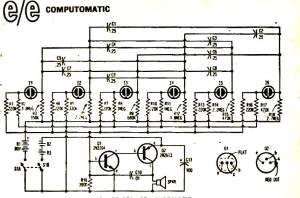
The first build-it-yourself project I opened to had several NE2 neon bulbs, some resistors and capacitors, a couple transistors and a battery. Looked simple without being too simple. The author, Herb Friedman (W2ZLF), described how the lights would blink in interesting ways, making great example of what some authors would have called an “idiot display”, pure blinkenlight fun, for little cost or effort. With bleepy chirpy sounds too.

“And soon the listener finds that exactly at the moment he thinks he has discovered the rhythm of the sound pattern, the light pattern makes a slight change and the sounds follow with a similar change in sequence. At one moment you may hear a clock inside
the box (accompanied by a glide tone), while the next moment your clock shifts into a sweep that mystifies.”

Great! I will build one.

While I already understood how one NE2 with one resistor and one capacitor worked to make a blinker, I couldn’t comprehend the messier network of this magazine project. Just what will it do?

Schematic that caught my interest when I was a kid

Schematic that caught my interest when I was a kid

I wondered what would happen if the capacitors were connected in other ways. Why six bulbs? What if we added a seventh – what would be good ways to add extra capacitors? I had only two maybe three NE2 bulbs taken out of old radios and whatever. I aimed to get a few more and build this gadget.

A PDF of the whole Jan/Feb ’69 issue is available at www.americanradiohistory.com

I never did build that thing – other projects became more important. Now that we live in an age of advanced computing and sophisticated FOSS software which anyone can have, who needs to build anything? We can simulate it on a computer.


(See my recently made Neon Blinker animation on Youtube)

A blinking light illustrates one of the simplest feature of a wave or any type of oscillation: repetition in time. The number of blinks per second, or per minute, is the frequency. The time between blinks is the period. Use whatever time unit is convenient.

frequency: how many blinks per second, or per minute.
period: how long it waits between blinks.

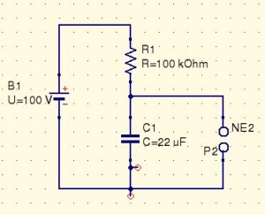
This circuit is the simplest oscillator one can build. Only three parts! (Besides the power source.)

Simple NE2 relaxation oscillator

Simple NE2 relaxation oscillator

How it works: Initially, there’s no charge on the capacitor. Charge from the power source flows through the resistor, accumulating in the capacitor. As the capacitor’s voltage rises, it eventually reaches the “breakdown voltage” (or “strike voltage”) of the neon bulb, typically around 80V to 90V but could be higher. This much voltage makes a strong enough electric field between the electrodes that electrons are peeled off their atoms, making a plasma. As electrons recombine with positive Ne+ ions, light is given off. Once started, the plasma does not require as much voltage to be maintained. Typically about 35V to 45V or so will be found across the bulb in typical use.

This glowing plasma conducts electricity, discharging the capacitor until its voltage drops to the extinction voltage of the neon bulb, {{V_e}}. At this point, the plasma dissipates, losing conductivity and glow, in only a millisecond becoming insulator. Then the cycle repeats, the resistor charging the capacitor as before.


So, what’s the simplest way to model an NE2 neon discharge lamp in SPICE?
I’m on Linux, using ngspice. Models can be found out there in the www, but I think it’d be more fun and educational to create something from scratch, starting simple and building it up.

The most important feature of the neon lamp is that is acts as a switch, normally off (infinite resistance) but can be on, with some nonzero resistance. The switch is turned on by a certain threshold voltage, then turns off at some lower extinction voltage. Basic hysteresis. Luckily, it happens that (afik) all flavors of SPICE have a standard switch component, “S”, which does everything we want. Although, instead of using S’s built-in Ron resistance parameter, we’ll use an explicit resistor in series, so we can diddle around with it later. NE2s aren’t exactly linear when on, but we’ll deal with that another day. For now, SPICE’s S will do fine for a basic first attempt at simulating an NE2 bulb.

BTW, if I didn’t mention already, I’m using ngspice-26 on a 64-bit quadcore Arch Linux machine.

First, the simplest rough NE2 model possible, in a file named neon001.sub

Neon NE2 super-simple version 001
* Lamp turns on at 80V, off at 40V, with on resistance given as model parameter

.model ne2sw  SW (Ron=41ohm VT=60V  VH=20V)

.SUBCKT Neon001  1  2
R1  1  11  45ohm
S  11 2   1 2   ne2sw
.ENDS

Then a circuit to use it, a simple RC flasher:

Testing NE2 models as simple one-bulb flasher
.include neon001.sub

Vpwr   Vplus  0   120V
R1     Vplus  2   220K
C1      2   20      2.2uF
RCmeas 20    0      1ohm     ; to measure current through C1
X1      2   21   Neon001
RNmeas 21    0   1ohm        ; to measure current in neon bulb
.end

Run a transient simulation in ngspice

tran  3msec 5sec  uic
plot v(2)
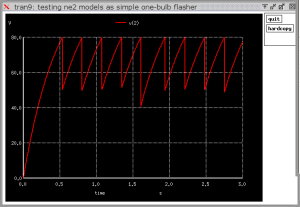
Voltage on capactor from SPICE simulation

Voltage on capactor from SPICE simulation

Odd, that one lower peak dropping down lower than the others. This is normal when the time step of a simulation is around the same size, or larger, than the time it takes for some fast process to occur. In this case, the discharging of the capacitor through the plasma-filled NE2 happens in less than a millisecond. The integrator using t_delta=3ms flies right over that, computing a system state after the event based on varying conditions at varying amounts of time before the event. With a 3ms step, it can’t accurately compute how much charge the capacitor loses.

Try a slightly different time step:

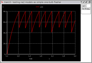
tran 3.1msec 3 uic
Capacitor voltage, slightly different time step.

Capacitor voltage, slightly different time step.

The pattern of lower peak variation is different. This is purely a simulator effect, nothing to do with real life. Since we are interested in simulating flasher circuits with multiple lights, it would be good to solve this problem. There’s about a 10V difference between the lowest of the low peaks and the highest of them. That amount of simulation error make useless any simulation of more complex circuits.

Two ways to solve this:
1. smaller time steps. This is easy. We get way more data, but our CPUs have not trouble dealing with that. 0.1ms might be good.
2. Modify the NE2 model to involve more capacitance, inductance, physical time delay effects of the plasma, so that the discharge process takes longer. Still, we need smaller time steps since 3ms was way too big.

tran 0.07msec 1.2 uic
plot v(2)
With smaller time step

With smaller time step

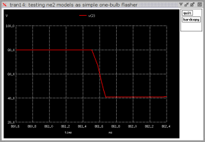
Tightly zoomed into a time span of a couple microseconds, we see how fast the discharge occurs. There are time steps within the discharge downslope. Probably not enough for accuracy, but we are glad that the curve bottoms out at 40V

Zoom-in of time axis showing discharge event

Zoom-in of time axis showing discharge event

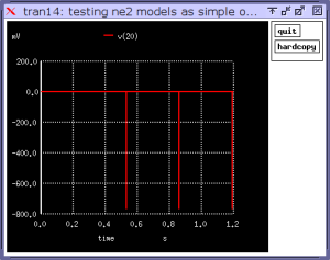
You may have noticed in the SPICE file that I had put a one-ohm resistor in series with the capacitor. We can plot the current flowing through the capacitor with it.

plot v(20)
Current flow in capacitor

Current flow in capacitor

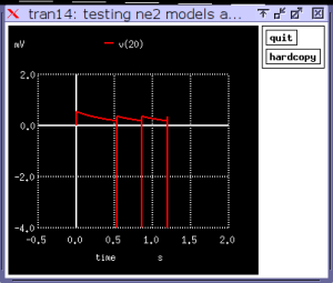
Current flow in capacitor, magnified to show it's positive, not zero, most of the time

Current flow in capacitor, magnified to show it’s positive, not zero, most of the time

The secone plot is zoomed in tight to a small voltage range, to show that the current is never zero, but positive as the capacitor charges for almost the entire cycle, and then briefly in 1/1000th the time discharges with a large current.

In switching and oscillating circuits like this, performing in a steady cycle, it’s normally a good rule of thumb (and physics) that the average current in each capacitor is zero.

An engineer building a neon discharge flasher like this would be wise to choose a type of capacitor which can handle the sudden reverse current flow, and have small ESR and lead inductance.

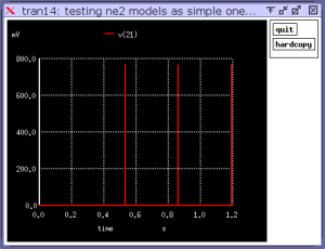
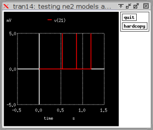
Another one-ohm resistor is in series with the neon bulb. By plotting v(21) and zooming in tight, we find zero current during most of the cycle, with

Current flow in the NE2

Current flow in the NE2

NE2 current, magnified. It really is zero most of the time.

NE2 current, magnified. It really is zero most of the time.

The average is not zero.  The NE2 is either off, like a piece of insulator, or it’s on, positive current flow for a brief time.

The important thing we have found with our crude NE2 model is that it works, but we must choose small time steps to avoid false variations of oscillation cycles.

I will write later about the basic NE2 multivibrator.

Pulse Waveforms and Harmonics

Recently on a Q&A forum, I answered some questions about pulse waveforms and harmonics.  This might be of interest to others, especially students in digital media or non-technical fields who need to have an idea about this math and related jargon.

In most fields of study, the duty cycle is the fraction of the whole period taken up by the high segment, often given as percentage.  A square wave is 50%.   A skinny spikey pulse might be 1%.    At least that’s how EEs and physicists talk, usually.

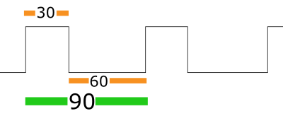
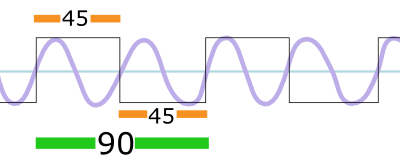
One could give the ratio of the high segment duration to the low segment. For this example I quickly drew up, the pulse width is 30 time units (nanoseconds, seconds, minutes, years, whatever), the gap between the pulses, where the signal is low, measures 60 time units, and the period of the signal is 90, the sum of those.    Note that the period is measured from the leading edge of one pulse to the leading edge of the next. We could measure trailing edge to trailing edge just as well, or from the center of a pulse to the center of the next.  Like studs in the wall of a house, one must be careful to specify and measure center-to-center, not the facing surface-to-surface air gaps between the pieces of lumber.

Pulse with 1/3 duty cycle.

Pulse with 1/3 duty cycle.

The time units are arbitrary, but we could say those are milliseconds.  A 90 ms period is the same as a frequency of 11 Hz, a tone so low only fish can hear it.  Argggh, a bad example then, but never mind.  We’ll carry on with this example, whether or not anyone can hear it.  Call the fundamental frequency f_0.   Period is seconds (or milliseconds) per cycle, while frequency is cycles per second.

The ratio of high to low is 1:2. This could also be described as 1/3 duty cycle, or 33% duty cycle. The high segment is in 1:3 ratio to the whole period. A sloppy writer might mention the 1:2 high-to-low ratio but not say so, misleading readers into thinking it’s high-to-whole and so they’re thinking it’s a square wave.

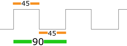
Here’s a square wave:

A square wve with 50% duty cycle

A square wve with 50% duty cycle

The high-to-low segment durations ratio is 1:1. The high segment is in 1:2 ratio with the whole.

Note that there’s really nothing “square” about a square wave. The horizontal axis is time, and the vertical axis is voltage, air pressure, the position of some point on a reed or string or whatever, which may be plotted with any units and scale you please. So there’s nothing going on involving four sides of equal length. It’s just an old convention that a 50% duty cycle pulse train like this is called “square” while otherwise, it’s  “rectangular”.


HARMONICS

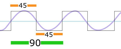
All waveforms may be thought of as sums of sine waves of many frequencies.  The most important sine wave component is the one with the same period as the waveforrm, the “Fundamental”.  For the square wave, it looks like this:

Fundamental sine component of a square wave.

Fundamental sine component of a square wave.

Fits nicely, doesn’t it?  Where the pulse is high, we see the sine is always positive. Its average  value in this segment is, oh, about +0.7 maybe.

Where the pulse is low, we think of that as providing an extra minus sign.  The sine is always negative there, averaging -0.7, but that extra minus sign flips it and gives overall another +0.7, for a total of +1.4.   This nonzero number tells us that this sine wave is a significant component of the square wave.

How about tripling the frequency of the sine wave?  Harmonic the Third.  Three complete cycles fit into the 90ms period.

Third harmonic of a square wave

Third harmonic of a square wave

An odd factoid about jargon – the harmonics are the frequencies higher than the fundamental.  We might think that the sine with twice the fundamental frequency, f = 2f_0, being the first of those, would be called the “first harmonic”, and f = 3f_0 the “second” and so on.  Indeed, some logic-minded authors write that way. But it’s confusing.  The far more common convention is to include the Fundamental as one of the harmonics.   The captain of a ship is still a member of the crew, right? That allows the numbers to match: f = 2f_0 is the “second harmonic”, f=29f_0 is the “twenty-ninth harmonic” and so on.  Much nicer!

So why is it common to refer to a fundamental frequency as f_0 instead of f_1? It is not the zeroth harmonic, is it?  But oh well.. Humans and their primitive math and illogical language…

Anyway, look at that three cycles-per-period harmonic.  What is the average value of the sine in the high pulse segment?  Look at the positive half cycles and negative half cycles.  In the high segment of the pulse, the first positive half cycle cancels out the first negative half cycle, leaving only the other positive half cycle remaining. It’s 1/3 the width of the positive half cycle we saw for the fundamental, so the resulting average value is 1/3 of what we had.  The low segment goes the same way, but negative, but then made positive by the extra negative sign due to being in the low segment.  

That’s why the third harmonic of a square wave is 1/3 the amplitude.   I leave it to you to sketch the fifth harmonic and become convinced that its average value is 1/5 of the fundamental.  So now you know where the 1/n harmonic series for square waves comes from.

I’m playing fast and loose here, doing by eye and hand-waving a crude Fourier Transform.  No proofs or equations or airtight arguments, but I hope the essential ideas are clear.


A LOPSIDED PULSE WAVEFORM

Let us look at that 1/3 duty cycle pulse from the start of this article.  We’ll look at the fundamental and the third harmonic, like we did for the square wave.

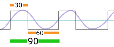
Pulse with 1/3 duty cycle, and its fundamental since wave.

Pulse with 1/3 duty cycle, and its fundamental since wave.

In the high segment, we have most of a positive half cycle. So the average value is positive (mumble-mumble) volts.  The low segment has all of the negative half cycle, and also  the intruding remaining part of the positive half cycle.  So we get some negative number, not as strong as for a square wave, and flip it to a positive value due to being in the low segment.  So we total up to some positive value, meaning that yes indeed the fundamental is an important contributor to the signal’s spectrum.


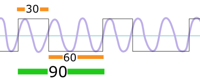
Now consider the third harmonic:

1/3 duty cycle pulse with its third harmonic

1/3 duty cycle pulse with its third harmonic

Three full cycles per period.  Hey looky here, this is interesting! In the high segment, we find one positive half cycle, and one negative half cycle. They cancel out. The average value is zero.  Likewise, we find zero in the low segment, although twice as much of it.   The average value of the third harmonic is flat zero — Harmonic the Third is *not* present in this particular pulse wave!

SQUARE WAVES HAVE NO EVEN HARMONICS

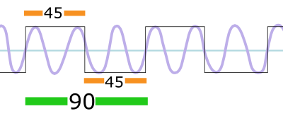
Going back to the square wave, we can see why the second harmonic, f=2f_0, zeros out, along with any even harmonic.

Square wave with its second harmonic

Square wave with its second harmonic

Each segment of the square wave holds exactly one full cycle of the harmonic sine wave, therefore averages out to zero.  If we  were looking at  the tenth harmonic, we’d find five full cycles of sine wave in each of the high and the low segments.


That’s it for now.  You are now a world-class expert on pulse waveforms and Fourier Transforms. Go forth and create and/or zero out harmonics!

(Illustrations (c) 2014 Daren Scot Wilson, created in Inkscape)

An Optimizer Bug in Clang

Found out about an interesting bug in Clang, the popular C++ compiler that aims to do better than GNU GCC.    But clang, with optimization turned on, may incorrectly optimize away useful code.

The problem, along with a short test program, is described in a question by Chris_F at StackOverflow,
 

When compiled with GCC, it works correctly, always returning an exit code of 6. When compiled with clang, with no opimization or the lowest level, we still get 6. But with -O2 or -O3, the clang-compiled executable is missing a bunch of stuff, to wit, everything, and returns 1 not 6.  

The following test program source is given by mukunda in the accepted answer. It’s shorter and simpler than the test program given in the question.   

— test.cpp —
// Test program – clang optimization bug
// compile with
//     g++ -o testgcc3 -O3  -std=gnu++11  test.cpp
// should return 6   (warning: run time is about half a minute)
// bug in clang:
//     clang -o testclang2 -O2  -std=c++11 test.cpp
// will return 6 for -O0 -O1 but returns 1 for -O2 -O3

#include <cstdint>
int main()
{
    uint32_t i = 0;
    uint32_t count = 1;
    while (1)
    {
        if( i < 5 )
            count+=1;
        if (i == 0xFFFFFFFF)
            break;
        i++;
    }
    return count; // should return 6
}
—- end of file —-

I compiled this with GCC 4.9.0 and Clang 3.4 each at four levels of optimization. The return values I saw were:

GCC -O0    6
GCC -O1    6
GCC -O2    6
GCC -O3    6
Clang -O0  6
Clang -O1  6
Clang -O2  1
Clang -O3  1

At least the erroneous versions return 1, which by convention indicates some sorta trouble, rather than 0.  

It has been discovered that using -fno-vectorize with clang makes the problem go away.  Some commenters think this bug a case of, or related to, http://llvm.org/bugs/show_bug.cgi?id=17288

I like clang overall, but stuff like this makes me nervous about compiling massive number crunching code with heavy optimizations, something we physicists like to do!

Quantum Mechanics for Engineers (Online book)

Stumbled upon an interesting site on quantum mechanics.  Aimed at engineers, and fine for others with a science background, it explains many of the important ideas of QM, with the math but without getting bogged down in math technicalities.  College level.  This is not  a pop-level work for the common people – it is for those who do have an engineering or science background, comfortable with calculus and scientific reasoning.   Reading this won’t get you a physics bachelor’s degree, but for, say, a mechanical engineer or systems engineer who had first year physics and maybe an advanced class or two from the physics department, and now needs to get up to speed on nano or semiconductors or photonics, this site offers a door of understanding into the quantum world.

Quantum Mechanics for Engineers – Leon van Dommelen

http://www.eng.fsu.edu/~dommelen/quantum/style_a/index.html


An Intuitive Description of Runge-Kutta Integration

(Based on a StackOverflow answer from November 2009)

Introduction

This may be a bit oversimplified so far as actual math, but is meant as an intuitive guide to how Runge Kutta integration works. RK integration is a numerical method for solving arbitrary first-order differential equations widely used by scientists, engineers, video game programmers, and everyone else who uses applied math beyond the simple.
Suppose we want to predict or simulate some physical system measured by some quantity y varying with time, y(t), for which we have an equation giving its rate of change

y'(t) = f(t,y)

For any time t and any value of y, the (simulated) forces or activities of the system determine a unique slope.

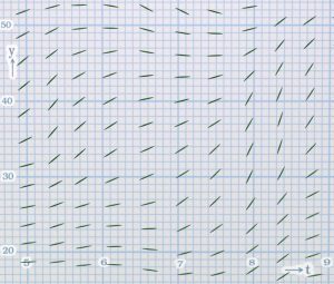
graph paper with many short sticks at angles suggesting  a field of slopes defined at all points

Slopes are given at every point in (t,y) space.

The function f(t,y) may be a simple algebraic function of t and y, or it may be a messier expression with exponentials and square roots and many terms. It may involve interpolating values given in a table. It may involve real-time data pouring in from gyrscopes, strain guages, photodiodes or other sensors.

Integration

With this kind of first-order differential equation, we are usually given an inital value y1 at some time t1. We want to know y at some later time t2.
From the differential equation, we can find the rate of change of y at t1. There is nothing else we can know for sure; everything else from here onward is guessing. We want to do a very good job of guessing.

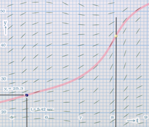
graph paper with pink curve, initial data point at t1, and indicator of final time point t2.

Setup of the basic integration problem. Try to find the value of the pink curve at t2, when you don’t already have the pink curve.

We cheat a bit here, and show the exact solution in pink. This will help us to judge how values computed numerically deviate from the ideal. In real life, we almost never have an exact solution to look at.

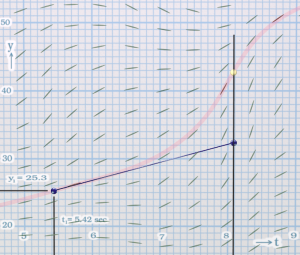
Euler integration is the simplest way to guess the future: linearly extrapolate from t1 to t2, using the precisely known slope and value of y at t1. This usually gives a bad answer. If t2 is far from t1, the linear extrapolation will fail to match any curvature in the ideal solution. If the step is too large, we might miss an intersting change in slope, an inflection point, or something. If we try to follow the ever-changing slopes more closely by taking many small steps from t1 to t2, we’ll have the problem of subtraction of similar values, resulting in roundoff errors, and it’ll take far more computational work to get to t2.

graph paper, initial point, and line segment from t1 to t2 angled to match slopes near initial point. At t2, it is nowhere near the pink curve.

Euler integration: One big linear extrapolation step determined only by information at the initial point. Euler sux!

If the differential equation happens to be very simple, like dy/dt = constant, cool, we actually have an exact answer. Real life is always more interesting than that and often nonlinear.
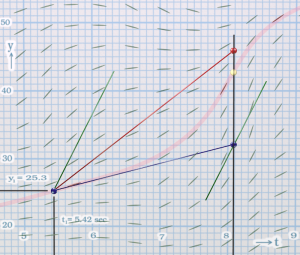
So we refine our guess. One way is to go ahead and do this linear extrapolation anyway, then hoping it’s not too far off from truth, use the differential equation to compute an estimate of the rate of change at t2. This, averaged with the (accurate) rate of change at t1, better represents the typical slope between t1 and t2 (shown in red below). We use this to make a fresh linear extrapolation from to t1 to t2. It’s not obvious if we should take the simple average, or give more weight to the more accurate slope at t1, without doing the math to estimate errors. Just note that there is a choice here. In any case, it’s a better answer than Euler gives.

graph paper, slopes, initial point, and three sloped lines showing how we can do slightly better than Euler.

How to do better than Euler: Take one normal Euler step (blue). Find the slope at t2 (green) and compare wih the initial slope (blue). Find their average for a “better” full step to t2 (red).

Making Half the Effort

Perhaps better, make our initial linear extrapolation to a point in time midway between t1 and t2, and use the differential equation to compute the rate of change there (blue). This gives roughly as good an answer as the average just described. Then use this mid-way slope for a better linear extrapolation from t1 to t2, since our purpose is to find the quantity at t2. This is the midpoint algorithm. It’s really no better than Euler.

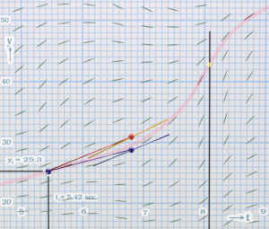
Finding the y value and slope at the midpoint depends on the slope at the initial point. We’d like to not be starting off in the wrong direction. What if we use this rough mid-point slope to make another linear extrapolation from t1 to the midpoint t? This is the red line in the figure below. It’s the same slope as the blue line, but relocated to the initial point t1,y1. With this, the differential equation gives us a better estimate of the slope at the halfway point. This lets us extrapolate once again from t1 all the way to t2 for a truly better answer. This is the Runge Kutta algorithm, at least a simple form of it.

graph paper, initial point at t1, and two sloped lines going only halfway to t2.

Maybe the slope at halfway across is better than averaging the initial and estimated final slope? Our first midpoint attempt (blue) can be used to obtain a better position at the midpoint (red and gold).

Could we do a third extrapolation to the midpoint? Sure, it’s not illegal, but detailed analysis shows diminishing improvement, such that other sources of error dominate the final result.

After that, we may compute the slope at t2, and somehow use that to better estimate how the the values and slopes of the ideal solution change with t. At this point, wordy hand-waving arguments and colorful sketches aren’t going to help. We need to do the algebra for fitting low-order polynomials to the values and slopes found by methods like we’ve described. Linear extrapolations and averages can only go so far. For true gains in quality we must consider 3rd and 4th order polynomials and tweak the details to obtain minimal errors.

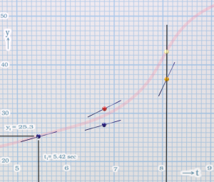
graph paper, initial point, curve, and four places marked. Sticks indicate slopes computed at all four spots.

The fourth-order RK computes slopes at four locations. Each location was determined from previous locations and their slopes.


Runge-Kutta Choices

The most popular form of fourth-order Runge Kutta uses the differential equation to compute the slope four times:

  1. at the intial point t1,
  2. twice at two in-between points,
  3. once at the final point t2.

The location of the in-between points are a matter of choice. We’ve illustrated having both at the midway point between t1 and t2. It is possible to choose points elsewhere, for example at one third of the way along and another at 2/3 of the way. The weights for averaging the four slopes will be different. In practice this doesn’t change things much, but may work slighty better for certain applied problems. Comparing different R-K algorithms applied to the same differential equation and initial data has a place in testing since, within errors that can be estimated, answers ought to agree.

Higher Orders, Lower Orders

Euler’s method is actually a first-order Runge Kutta method. R-K covers a range of methods to choose from. You don’t want first-order, as every beginner at numerical integration discovers from experimenting with Euler. Higher order methods are better, up to fourth order. Beyond that, the extra effort rarely pays off in performance.

Remember that beside the integration method, there is the choice of step size. Higher order RK methods allow you to take longer steps, therefore fewer steps. While there’s more computational work at each step, it’s less work overall to get from t1 to t2.

Original Inspiration

The essence of the  original question, which won a  Notable Question badge, is:

Can anybody explain in simple terms how RK4 works? Specifically, why are we averaging the derivatives at 0.0f, 0.5f, 0.5f, and 1.0f? How is averaging derivatives up to the 4th order different from doing a simple euler integration with a smaller timestep?


Introduction and Intent

This blog will be all about waves in the physical world.  We will look at musical instruments, drumhead shapes, missing neutrinos, quantum mechanics, microwave antennas, and much more.

Everything is described by waves, undulations, cycles.  This universal feature of reality ties things together, unifies our theories of physics, but also there is tremendous variety to enjoy – just ask: what is it that’s doing the waving?  It could be air, water, networks of steel beams, DNA molecules, quantum particles that barely exist, or huge swarms of stars in the spiral arms of galaxies. It could even be the Big Bang as we see it now with radio telescopes, 13.6 billion years after it happened.

The level of presentation will include math, physics and illustrations.  The intended audience will be broad, from high schoolers who love math and physics to professors and engineers.  Visitors with no scientific background at all are also welcome, and may get something out of most of these posts even if skipping over the math.  Most of the material is developed intuitively, with visuals, not theorems and proofs like in textbooks.  Abstract ideas will be illustrated with something you can look at.

On occasion there may be a post with seriously deep world-class PhD research and esoteric math, but even then I’ll aim to put in clear explanations, colorful fun diagrams and animations to entertain everyone in the lower 99.99% of intellect. Some days, I may go the opposite and write about very basic math ideas.  It’s my blog, and so I can do that.

Who am I?  I took apart mechanical and electrical toys as a kid, was fascinated by the insides of the TV when my Dad checked the vacuum tubes, read every book in the public library on electronics – both of them – and loved astronomy and math.  My first word was “light” and I have always enjoyed light and shadow, colors, shapes.  I majored in Physics at Oakland University then went into graduate studies in the same field at Indiana University.  Some companies and research organizations I’ve worked at or did some project for include NRAO, University of Central Florida, Space Science Institute, Stanford Linear Accelerator Center, and Chrysler.  If I’m not doing electronics or image processing, I’m paying the rent by doing software work for scientists and engineers..

Besides physics, math and software, I also have worked in live and recorded television production, played in a church bell choir, did a bit of theatrical dance in Ann Arbor, played sax in a community band for a smaller city in New Mexico, and soon hope to begin surfing near Del Mar, Solana or Encinitas California.  All these activities involve waves, and in more than one way.

It thrills me to relate theoretical physics to everyday reality, to apply math to art and fun and nature.  I’d like to explain to you, as clearly as I can, how the math and physics of waves apply to so many things in our lives.